[BLOG] How does DSP work? [Part 2]

[griffinboy]

How does DSP work? [Part 2]

Welcome back!

In the previous part, we saw that audio effects work by changing sample values.
And we saw that a volume effect is just multiplication.

Next you might be wondering: how does something like a filter work?
That's the question we are going to answer today.

We're going to start with the simplest example of a filter: a smoother.

A smoother is a low pass filter in its simplest form.
The reason will become clear as we build one.

Low pass filter

You probably already know that a low-pass filter removes high frequencies.

But inside a DSP effect, the audio waveform is just a block of sample values:

[0.14,  0.21,  0.08,  0.29,  -0.04,  -0.18,  -0.11,  -0.32,  ...]

Those numbers are the waveform.
So how are we supposed to alter these sample values to remove high frequencies?
let me explain:

---

You probably already know that frequency is how fast a waveform is.

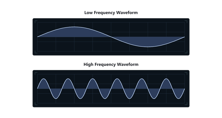
And of course, a waveform can contain many frequencies at once.
For example, if we add two waves together: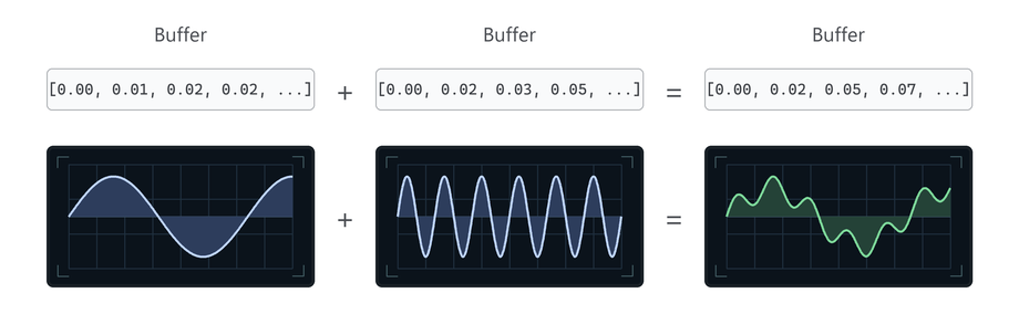

We get a wave that contains high and low frequencies.

So how do we remove the high frequencies from this kind of wave?

Let's demonstrate with a complex wave.
Here is a waveform with plenty of high-frequency content: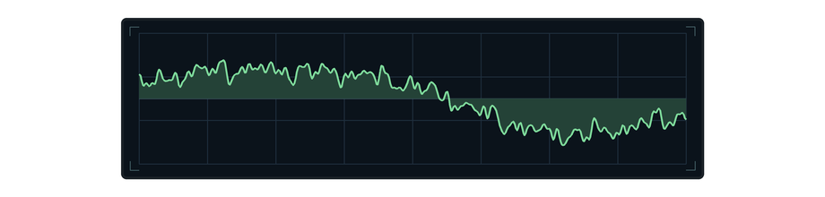

The broad sine-like shape is low frequency.
The fine, noisy-looking details are higher frequencies.

Now watch what happens when we low-pass the sound:

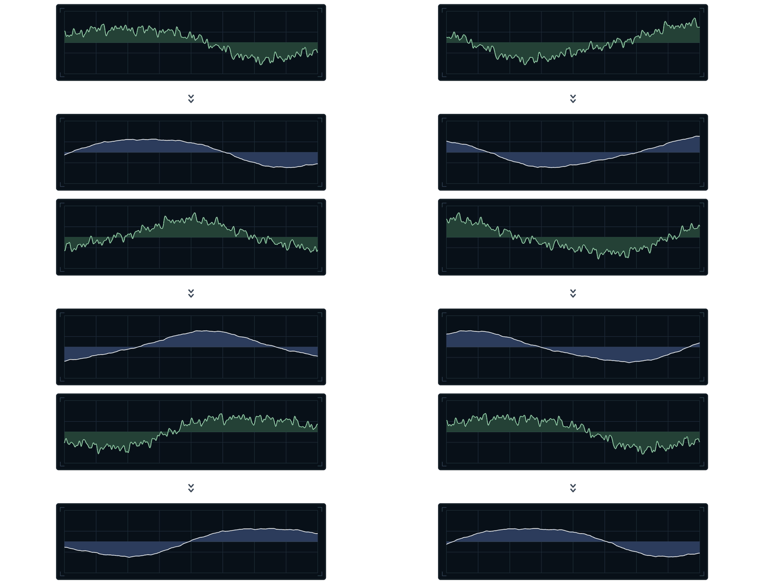
The noisy detail is removed, while the broad low-frequency shape remains.

The waveform looks smoothed! A smoothing algorithm can remove the high frequencies!

A Smoother

So let's look at how a smoother works.

[My explanation may be a little hard to follow - bear with me please! I will try and explain it in a few different ways]

There are many ways to write a smoother.
The version we're going to use generates a new, smoothed waveform in place of the original one.

The algorithm works like this:
Every sample, look at the original waveform sample, and move our new waveform sample (the smoothed waveform) towards it.
But only move it a small amount each sample.

Here is an animation that shows the algorithm in action:

Green is the original waveform sample value.
Blue is our smoothed waveform we are creating.

We use the green as a "target", and our smoothed value will move towards it over time.

Notice how the original (Green) instantly moves to the new sample value, while our smoothed (Blue) value takes a while to catch up.

Basically, it's incapable of moving fast!
In other words... it can't be high frequency. Only low frequency!

Here is the same process running from sample to sample, on a (very zoomed in) waveform:

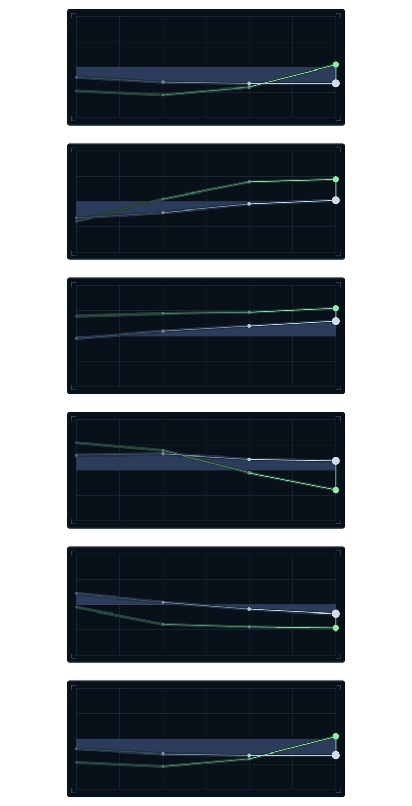
At the right edge, green is the current sample of the original waveform, and blue is our smoothed value.

The smoothing algorithm works by starting from the previous blue value, and then moving towards the green target sample value.

The resulting smoothed waveform is basically a slow, tired version of the original wave.
It can follow the broad movements, but it can't keep up with quick details

The algorithm looks like this:

var green;

for each sample in the chunk:
    move the green value partway towards the current sample
    output the green value

The Math

Now let's write the smoothing algorithm as pseudocode:

amount = 0.1
smoothedValue = 0.0

for each sample in the chunk:
    smoothedValue = lerp(smoothedValue, sample, amount)
    sample = smoothedValue

smoothedValue is the current height of the blue waveform.
It starts at 0.0, and it is kept after each sample so that the next calculation can continue from the same height.

For each sample, lerp moves smoothedValue towards the height of the original waveform.
The amount controls how far it is allowed to move.

An amount of 1.0 reaches the original sample value immediately.
An amount of 0.1 only moves one tenth of the distance.

lerp is short for a linear interpolation function.
In this case, it calculates a new sample value (height) between the current smoothedValue and the original sample.

The calculation inside lerp is:

smoothedValue += (sample - smoothedValue) * amount

sample - smoothedValue measures the distance between the blue value and the green target.
Multiplying that distance by amount chooses how much of the distance to travel.
Adding the result to smoothedValue moves the blue value towards the green one.

Finally, we output the smoothedValue.

Because every calculation continues from the value calculated for the previous sample, repeating this process across the waveform for every sample in the buffer, produces exponential smoothing.

In HISE-Style C++

The same calculation in C++ looks like this:

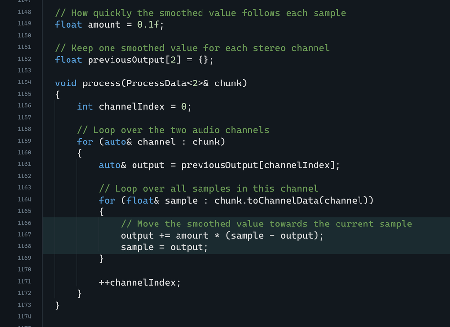
Some trivia:
That stored value is called the filter's state.
Because each result depends on the result from the sample before it, this is a recursive filter, also called an IIR filter.
With one stored value per channel, this particular algorithm is called a one-pole low-pass filter.

Cutoff Frequency

Our example code uses a fixed amount of 0.1.

If we set amount to 1.0, the smoothed value reaches every sample immediately.
Nothing is smoothed.

With a smaller amount, the smoothed value takes longer to reach each sample:
The smoothed value changes more slowly, so more high-frequency detail is flattened.

When this calculation is used in an audio filter effect, the control is normally presented as a cutoff frequency in Hz.
This is done using some extra conversion math.
The cutoff frequency and Daw sample rate are then converted into the amount used by the code.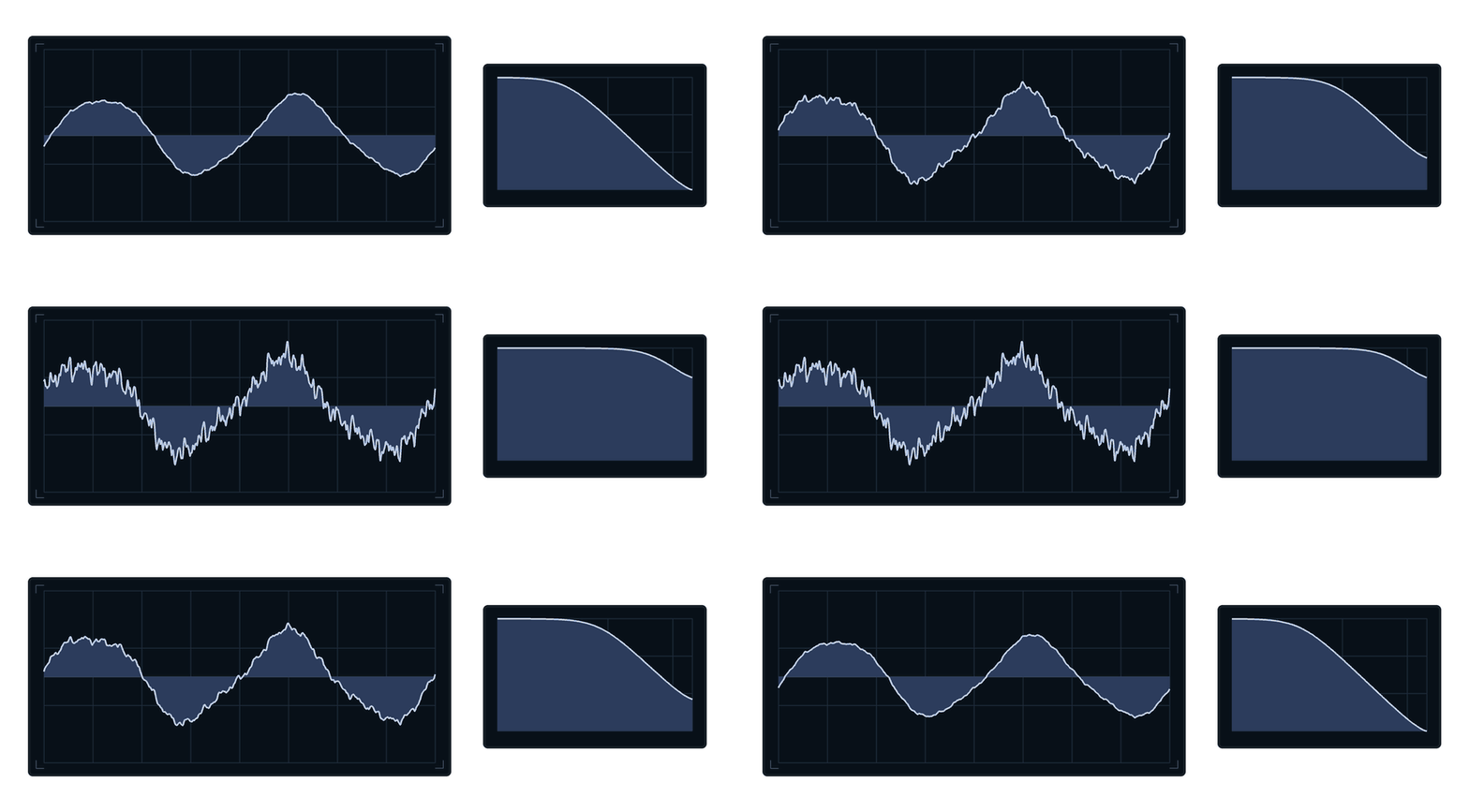

^ The smoother with changing amount (cutoff):

At a low cutoff, the blue waveform loses most of its fine detail.
As the cutoff rises, the blue waveform follows more of the detail.

Other Audio Filters

The smoother I showed you is a real one-pole low-pass filter.
Its slope is a gentle 6 dB per octave!

But audio filters can also have steeper slopes, resonance, and completely different shapes:

Different filter calculations produce different frequency responses:

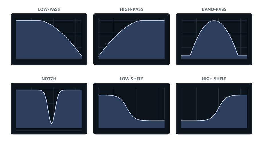
More advanced filters store more values, and combine them in different ways.

Two useful names to look for are state-variable filters and biquad filters.
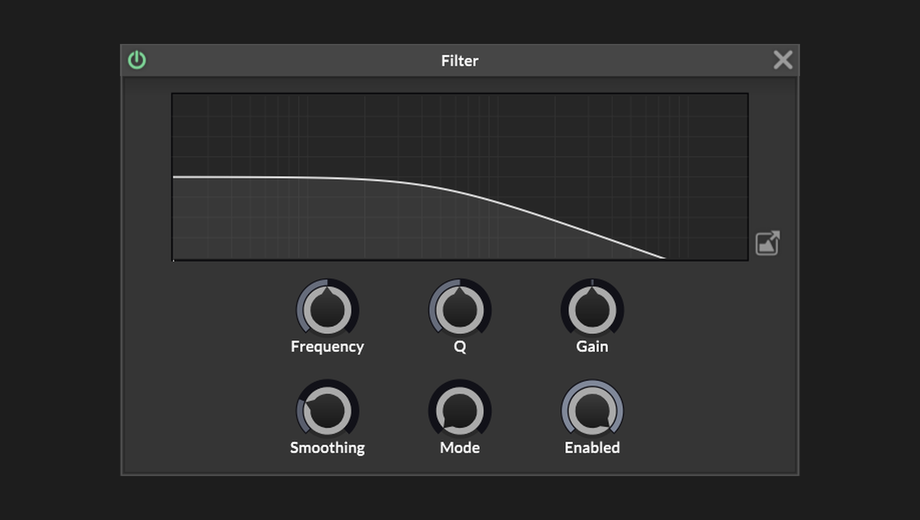
You can find the algorithms for these online, and they are also implemented in HISE's Filter node.

HISE provides a state-variable filter node.
MusicDSP's Chamberlin state-variable filter provides a compact explanation and working algorithms for SVF filters.
The Audio EQ Cookbook contains the standard equations for many familiar EQ filter shapes.

To Recap

Inside a DSP effect, the audio waveform is made up of chunks of sample values.

For a one-pole smoother, each sample we calculate a new value partway between its previous result and the incoming sample.

This adds resistance to fast changes, and suppresses the fine detail in the waveform.

That "fast detail" contains high-frequency content, so the high frequencies become quieter when we do this.

[David Healey]

@griffinboy Thanks for this. Put a link to part 1 at the top.